

How To Check If Gdal Is Installed
- Introduction
- Get the Data Package
- Software
- GDAL
- Windows
- Mac/Linux
- QGIS
- GDAL
- Getting Familiar with the Command Prompt
- Windows
- Mac/Linux
- ane. GDAL Tools
- 1.one Basic Raster Processing
- one.1.1 Merging Tiles
- Do ane
- 1.1.ii Converting Formats
- 1.1.iii Compressing Output
- 1.1.four Setting NoData Values
- ane.1.5 Wrting Cloud-Optimized GeoTIFF (COG)
- 1.ii Processing Elevation Data
- i.2.1 Creating Hillshade
- 1.2.two Creating Color Relief
- Exercise 2
- ane.three Processing Aerial Imagery
- one.iii.ane Create a preview image from source tiles
- 1.three.2 Create a Tile Index
- 1.three.three Mosaic and prune to AOI
- 1.3.5 Creating Overviews
- 1.4 Processing Satellite Imagery
- 1.4.ane Merging individual bands into RGB composite
- 1.4.2 Apply Histogram Stretch and Color Correction
- 1.four.3 Raster Algebra
- Exercise iii
- one.iv.4 Pan Sharpening
- 1.5 Processing WMS Layers
- 1.5.1 List WMS Layers
- ane.5.two Creating a Service Clarification File
- 1.5.3 Downloading WMS Layers
- ane.6 Georeferencing
- 1.vi.1 Georeferencing Images with Bounding Box Coordinates
- ane.6.ii Georeferencing with GCPs
- Assignment
- 1.one Basic Raster Processing
- two. OGR Tools
- ii.ane ETL Basics
- ii.i.1 Read a CSV data source
- 2.1.2 Convert it to indicate data layer
- 2.1.3 Assign it a CRS
- two.1.4 Extract a subset
- two.one.5 Modify the information type of a column
- 2.one.6 Rename the layer in GeoPackage.
- Practice 4
- two.2 Merging Vector Files
- Practise 5
- 2.3 Geoprocessing and Spatial Queries
- 2.iii.1 Reprojecting Vector Layers
- 2.iii.ii Creating Buffers
- 2.three.three Performing Spatial Queries
- 2.iii.4 Data Cleaning
- ii.ane ETL Basics
- 3. Running commands in batch
- four. Automating and Scheduling GDAL/OGR Jobs
- Tips for Improving Performance
- Configuration Options
- Multithreading
- Supplement
- Creating Contours
- Creating Colorized Hillshade
- Removing JPEG Compression Artifacts
- Splitting a Mosaic into Tiles
- Merging Files with Unlike Resolutions
- Summate Pixel-Wise Statistics over Multiple Rasters
- Raster to Vector Conversion
- Working with KML Files
- Exporting Information to KML files
- Converting KML Files to Other Formats
- KML vs. LIBKML Drivers
- Extracting Epitome Metadata and Statistics
- Using Virtual Layers
- Read Geonames Files
- Applying Filters
- Merging Files
- Resources
- Data Credits
- License
![]()
Introduction
GDAL is an open up-source library for raster and vector geospatial data formats. The library comes with a vast collection of utility programs that can perform many geoprocessing tasks. This class introduces GDAL and OGR utilities with example workflows for processing raster and vector data. The class too shows how to use these utility programs to build Spatial ETL pipelines and do batch processing.

View the Presentation
Get the Data Package
The code examples in this course use a diversity of datasets. All the required datasets are supplied to you in the gdal_tools.zippo file. Unzip this file to the Downloads directory. All commands below presume the data is available in the <home folder>/Downloads/gdal_tools/ directory.
Not enrolled in our instructor-led course but want to piece of work through the material on your own? Become complimentary access to the data package
Software
This course requires installing the GDAL package. Forth with GDAL, we highly recommend installing QGIS to view the result of the control-line operations. You will notice installation instructions for both the software below.
GDAL
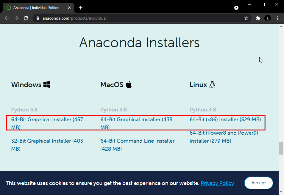
The preferred method for installing the GDAL Tools is via Anaconda. Follow these steps to install Anaconda and the GDAL library.
Download the Anaconda Installer for Python 3.7 (or a higher version) for your operating system. Once downloaded, double click the installer and install it into the default suggested directory.
Note: If your username has spaces, or not-English language characters, information technology causes problems. In that instance, yous tin can install it to a path such as C:\anaconda.
Windows
Once Anaconda installed, search for Anaconda Prompt in the Commencement Carte du jour and launch a new window.
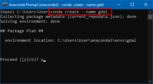
- Create a new surround named
gdal. When prompted to confirm, blazonyand printing Enter.
conda create --name gdal Note: You tin select Correct Click → Paste to paste commands in Anaconda Prompt.
- Actuate the environment and install the
gdalpackage. When prompted to confirm, typeyand press Enter.
conda activate gdal conda install -c conda-forge gdal 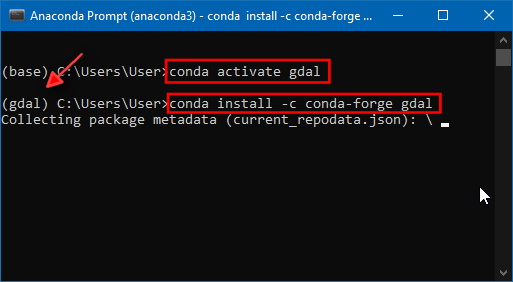
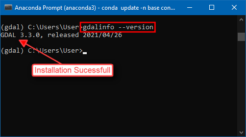
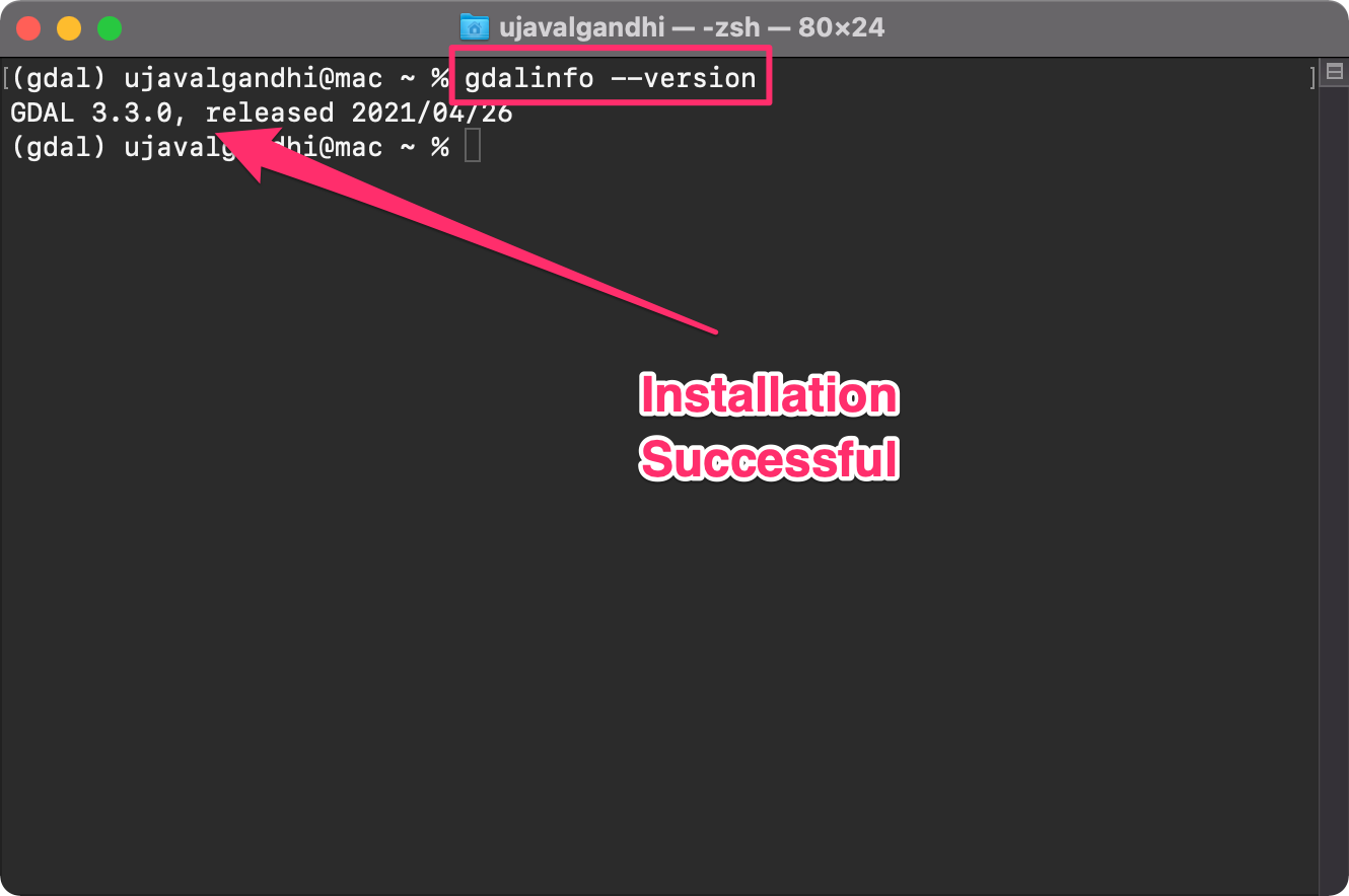
- Once the installation finishes, verify if you are able to run the GDAL tools. Type the following command and bank check if a version number is printed.
gdalinfo --version The version number displayed for you lot may exist slightly unlike. As long every bit you practice not get a
command non constitutemistake, you should be set for the class.
Mac/Linux
Once Anaconda is installed, launch a Concluding window.
- Create a new environment named
gdal. When prompted to confirm, typeyand printing Enter.
conda create --name gdal 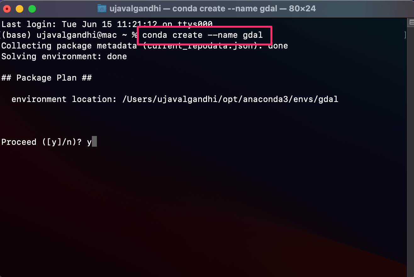
- Actuate the environs and install the
gdalpackage. When prompted to confirm, typeyand press Enter.
conda actuate gdal conda install -c conda-forge gdal 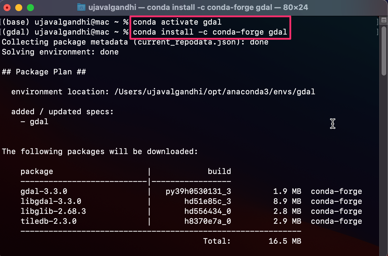
- Once the installation finishes, verify if you are able to run the GDAL tools. Blazon the following command and check if a version number is printed.
gdalinfo --version The version number displayed for y'all may be slightly unlike. As long as y'all do not get a
command not founderror, you should be fix for the grade.
QGIS
This course uses QGIS LTR version iii.16 for visualization of results. Information technology is not mandatory to install QGIS, but highly recommended.
Please review QGIS-LTR Installation Guide for step-by-step instructions.
Getting Familiar with the Command Prompt
All the commands in the exercises below are expected to be run from the Anaconda Prompt on Windows or a Terminal on Mac/Linux. We will now cover basic terminal commands that will aid you get comfortable with the environment
Windows
| Control | Clarification | Example |
|---|---|---|
cd | Change directory | cd Downloads\gdal-tools |
cd .. | Change to the parent directory | cd .. |
dir | Listing files in the current directory | dir |
del | Delete a file | del test.txt |
rmdir | Delete a directory | rmdir /s exam |
mkdir | Create a directory | mkdir test |
type | Print the contents of a file | type test.txt |
> output.txt | Redirect the output to a file | dir /b > test.txt |
cls | Clear screen | cls |
Mac/Linux
| Control | Description | Example |
|---|---|---|
cd | Change directory | cd Downloads/gdal-tools |
cd .. | Change to the parent directory | cd .. |
ls | List files in the current directory | ls |
rm | Delete a file | rm examination.txt |
rm -R | Delete a directory | rm -R exam |
mkdir | Create a directory | mkdir test |
cat | Print the contents of a file | cat test.txt |
> output.txt | Redirect the output to a file | ls > test.txt |
clear | Clear screen | clear |
3. Running commands in batch
You can run the GDAL/OGR commands in a loop using Python. Say yous want to catechumen the format of the images from JPEG200 to GeoTiff. You would run a command such as below.
gdal_translate -of GTiff -co Shrink=JPEG {input} {output} Just it would exist a lot of manual effort if you want to run the commands on hundreds of input files. Here'due south where a simple python script tin can assist you automate running the commands in a batch. The data directory contains a file called batch.py with the following python code.
import os input_dir = 'naip' command = 'gdal_translate -of GTiff -co Compress=JPEG {input} {output} ' for file in bone.listdir(input_dir): if file.endswith('.jp2'): input = os.path.join(input_dir, file) filename = os.path.splitext(os.path.basename(file))[0] output = bone.path.bring together(input_dir, filename + '.tif') bone.arrangement(command.format(input = input, output=output)) In Anaconda Prompt, run the following control from gdal-tools directory to start batch processing on all tiles contained in the naip/ directory.
python batch.py The data directory too contains an example of running the batch commands in parallel using python'due south built-in multiprocessing library. If your system has multi-core CPU, running commands in parallel similar this on multiple threads tin give yous performance boost over running them in serial.
import os from multiprocessing import Pool from timeit import default_timer as timer input_dir = 'naip' command = 'gdal_translate -of GTiff -co Shrink=JPEG {input} {output} ' def process(file): input = bone.path.join(input_dir, file) filename = os.path.splitext(os.path.basename(file))[0] output = os.path.join(input_dir, filename + '.tif') bone.system(command.format(input = input, output=output)) files = [file for file in bone.listdir(input_dir) if file.endswith('.jp2')] if __name__ == '__main__': start = timer() p = Puddle(4) p.map(procedure, files) end = timer() print(cease - starting time) commencement = timer() for file in files: process(file) cease = timer() print(end - start) The script runs the commands both in parallel and series mode and prints the time taken by each of them.
python batch-parallel.py 4. Automating and Scheduling GDAL/OGR Jobs
The easiest way to run commands on a schedule on a Linux-based server is using a Cron Job.
You will take to edit your crontab and schedule the execution of your script (either Beat out Script or Python Script). The key is to actuate the conda surroundings earlier execution of the script.
Bold you lot have created a script to execute some GDAL/OGR commands and placed it at /usr/local/bin/batch.py, here'south a sample crontab entry that executes it every forenoon at 6am.
0 half-dozen * * * conda activate gdal;python /use/local/bin/batch.py; conda conciliate If yous get an error while execution, yous may have to include some environs variables in the crontab file so information technology can detect conda correctly. Learn more.
SHELL=/bin/fustigate BASH_ENV=~/.bashrc 0 6 * * * conda activate gdal;python batch-parallel.py; conda deactivate Tips for Improving Functioning
Configuration Options
GDAL has several configuration options that can be tweaked to help with faster processing.
-
--config GDAL_CACHEMAX 512: This option is the 1 that helps speed upwardly well-nigh GDAL commands by assuasive them to apply larger amount of RAM (512 MB) reading/writing data. -
--config GDAL_NUM_THREADS ALL_CPUS: This option helps speed up write speed by using multiple threads for compression. -
--debug on: Turn on debugging mode. This prints additional data that may help you find performance bottlenecks.
Multithreading
gdalwarp utility supports multithreaded processing. There are two different options for parallel processing.
-
-multi: This option parallelizes I/O and CPU operations. -
-wo NUM_THREADS=ALL_CPUS: This option parallelizes CPU operations over several cores.
In that location is also another option that allows gdalwarp to employ more RAM for caching. This option is very helpful to speed upward operations on big rasters
-
-wm: Ready a higher memory for caching
All of these options can be combined that may outcome in faster processing of the data.
gdalwarp -cutline aoi.shp -crop_to_cutline naip.vrt aoi.tif -co Shrink=JPEG -co TILED=Aye -co PHOTOMETRIC=YCBCR -multi -wo NUM_THREADS=ALL_CPUS -wm 512 --config GDAL_CACHEMAX 512 Supplement
Creating Contours
Note : The
merged.tiffile used below was created in the Merging Tiles section.
The GDAL bundle comes with the utility gdal_countour that creates profile lines and polygons from DEMs.
You tin can specify the interval between contour lines using the -i option.
gdal_contour merged.tif contours.gpkg -i 500 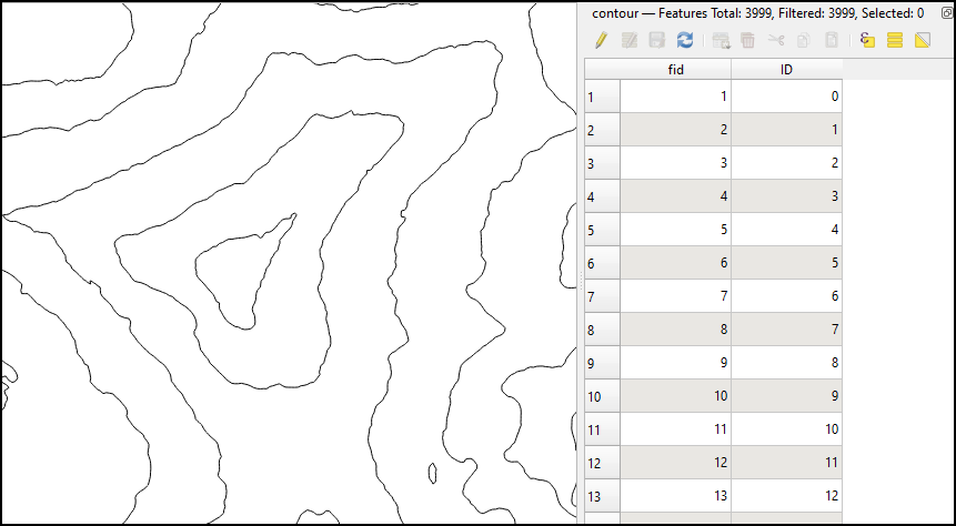
Contour Lines from DEM
Running the command with default options generates a vector layer with contours just they do not take any attributes. If yous want to label your contour lines in your map, you may desire to create contours with elevation values as an attribute. You tin can use the -a option and specify the name of the attribute.
gdal_contour merged.tif contours.gpkg -i 500 -a elev 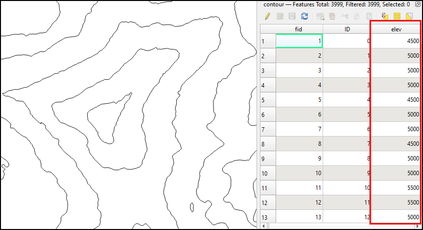
Profile Lines with Superlative Attribute
You tin likewise create polygon contours. Polygon contours are useful in some applications such as hydrology where you lot want to derive average depth of rainfall in the region between isohyets. You can specify the -p option to create polygon contours. The options -amin and -amax can exist provided to specify the aspect names which will store the min and max elevation for each polygon. The command below creates a profile shapefile for the input merged.tif DEM.
gdal_contour merged.tif contour_polygons.shp -i 500 -p -amin MINELEV -amax MAXELEV 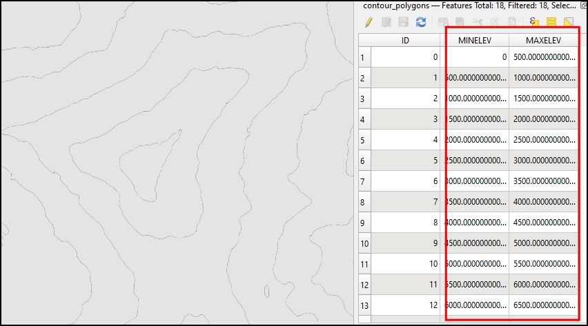
Profile Polygons with Peak Attributes
Creating Colorized Hillshade
If you lot want to merge hillshade and color-relief to create a colored shaded relief map, you tin can use use gdal_calc.py to create do gamma and overlay calculations to combine the two rasters. 1
gdal_calc.py -A hillshade.tif --outfile=gamma_hillshade.tif \ --calc="uint8(((A / 255.)**(ane/0.5)) * 255)" gdal_calc.py -A gamma_hillshade.tif -B colorized.tif --allBands=B \ --calc="uint8( ( \ 2 * (A/255.)*(B/255.)*(A<128) + \ ( 1 - two * (1-(A/255.))*(one-(B/255.)) ) * (A>=128) \ ) * 255 )" --outfile=colorized_hillshade.tif 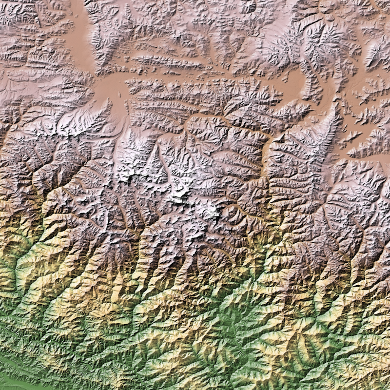
Colorized Shaded Relief
Removing JPEG Compression Artifacts
Applying JPEG pinch on aeriform or drone imagery can crusade the results to have edge artifacts. Since JPEG is a lossy compression algorithm, it causes no-information values (typically 0) beingness converted to non-zero values. This causes problems when you want to mosaic different tiles, or mask the black pixels. Fortunately, GDAL comes with a handy tool chosen nearblack that is designed to solve this problem. Y'all tin specify a tolerance value to remove border pixels that may not be exactly 0. It scans the image in till information technology finds these well-nigh-black pixel values and masks them. Permit's say we want to accept the mosaic created in the Moasic and Prune to AOI section and mask the black pixels. If we but gear up 0 as nodata value, yous will cease upwardly with edge artifacts, along with many night pixels within the mosaic (building shadows/water etc.) being masked. Instead we utilize the nearblack program to set edge pixels with value 0-5 existence considered nodata.
nearblack -near five -setmask -o aoi_masked.tif aoi.tif \ -co COMPRESS=JPEG -co TILED=Yes -co PHOTOMETRIC=YCBCR 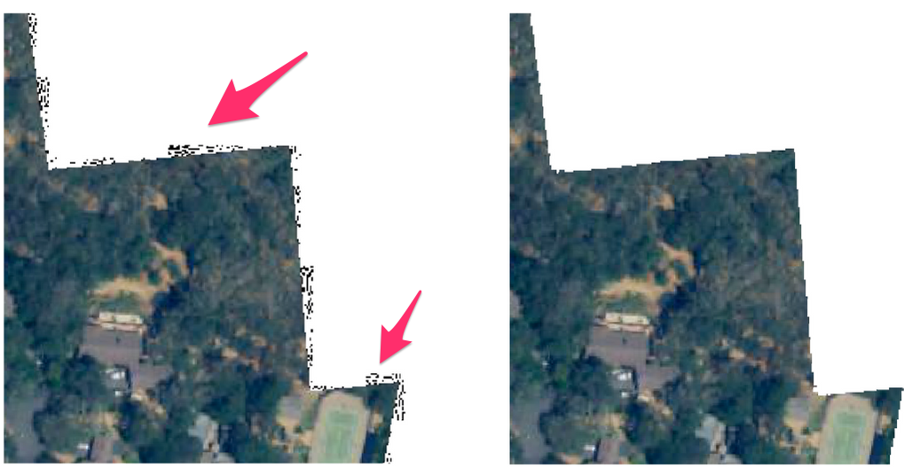
JPEG Artifacts Cleaned by GDAL nearblack
Splitting a Mosaic into Tiles
When delivering large mosaics, it is a skillful idea to dissever your large input file into smaller chunks. If you lot are working with a very large mosaic, splitting it into smaller chunks and processing them independently can assistance overcome memory bug. This is also helpful to prepare the satellite imagery for Deep Learning. GDAL ships with a handy script called gdal_retile.py that is designed for this chore.
Let's say we have a big GeoTIFF file aoi.tif and want to split it into tiles of 256 x 256 pixels, with an overlap to 10 pixels.
Beginning nosotros create a directory where the output tiles will be written.
mkdir tiles Nosotros can at present use the following command to split the file and write the output to the tiles directory.
gdal_retile.py -ps 256 256 -overlap 10 -targetDir tiles/ aoi.tif This will create smaller GeoTiff files. If you want to railroad train a Deep Learning model, you would typically require JPEG or PNG tiles. You tin batch-convert these to JPEG format using the technique shown in the Running Commands in batch department. Since JPEG/PNG cannot concord the georeferencing information, we supply the WORLDFILE=YES creation option.
gdal_translate -of JPEG <input_tile>.tif <input_tile>.jpg -co WORLDFILE=YES This will create a sidecar file with the .wld extension that volition shop the georeferencing information for each tile. GDAL will automatically employ the georeferencing information to the JPEG tile as long this file exists in the aforementioned directory. This mode, yous can make inference using the JPG tiles, and utilize the .wld files with your output to automatically georeference and mosaic the results.
Merging Files with Different Resolutions
If you had a agglomeration of tiles that you lot wanted to merge, merely some tiles had a different resolution, you lot tin utilize specify the -resolution flag with gdalbuildvrt to ensure the output file has the expected resolution.
Continuing the instance from the Processing Aerial Imagery section, nosotros can create a virtual raster and specify the resolution flag
gdalbuildvrt -input_file_list filelist.txt naip.vrt -resolution highest -r bilinear Translating this file using gdal_translate or subsetting it with gdalwarp will result in a mosaic with the highest resolution from the source tiles.
Calculate Pixel-Wise Statistics over Multiple Rasters
gdal_calc.py can compute pixel-wise statistics over many input rasters or multi-ring rasters. Starting GDAL v3.three, it supports the total range of numpy functions, such as numpy.average(), numpy.sum() etc.
Here'due south an example showing how to compute the per-pixel total from 12 different input rasters. The prism folder in your data parcel contains 12 rasters of atmospheric precipitation over the continental U.s.a.. We volition compute pixel-wise full precipitation from these rasters. When you read multiple rasters using the same input flag -A, gdal_calc.py creates a 3D numpy array. It can then be reduced along the centrality 0 to produce totals.
cd prism gdal_calc.py \ -A PRISM_ppt_stable_4kmM3_201701_bil.bil \ -A PRISM_ppt_stable_4kmM3_201702_bil.bil \ -A PRISM_ppt_stable_4kmM3_201703_bil.bil \ -A PRISM_ppt_stable_4kmM3_201704_bil.bil \ -A PRISM_ppt_stable_4kmM3_201705_bil.bil \ -A PRISM_ppt_stable_4kmM3_201706_bil.bil \ -A PRISM_ppt_stable_4kmM3_201707_bil.bil \ -A PRISM_ppt_stable_4kmM3_201708_bil.bil \ -A PRISM_ppt_stable_4kmM3_201709_bil.bil \ -A PRISM_ppt_stable_4kmM3_201710_bil.bil \ -A PRISM_ppt_stable_4kmM3_201711_bil.bil \ -A PRISM_ppt_stable_4kmM3_201712_bil.bil \ --calc='numpy.sum(A, centrality=0)' \ --outfile total.tif Currently, gdal_calc.py doesn't support reading multi-ring rasters as a 3D array. So if you want to apply a similar computation on a multi-band raster, y'all'll have to specify each band separately. Permit's say, we want to summate the pixel-wise boilerplate value from the RGB blended created in the Merging individual bands into RGB composite department. We can use the command as follows.
gdal_calc.py \ -A rgb.tif --A_band=1 \ -B rgb.tif --B_band=2 \ -C rgb.tif --C_band=3 \ --calc='(A+B+C)/three' \ --outfile hateful.tif Raster to Vector Conversion
GDAL comes with the gdal_polygonize.py allowing u.s.a. to convert rasters to vector layers. Allow's say we want to extract the coordinates of the highest elevation from the merged raster in the Merging Tiles section. Querying the raster with gdalinfo -stats shows united states that the highest pixel value is 8748.
We can use gdal_calc.py to create a raster using the condition to friction match just the pixels with that value.
gdal_calc.py --calc 'A==8748' -A merged.vrt --outfile everest.tif --NoDataValue=0 The result of a boolean expression like above will be a raster with 1 and 0 pixel values. Every bit nosotros set the NoData to 0, we only have 1 pixel with value 1 where the condition matched. We can convert information technology to a vector using gdal_polygonize.py.
gdal_polygonize.py everest.tif everest.shp If we want to extract the centroid of the polygon and impress the coordinates, we can use ogrinfo command.
ogrinfo everest.shp -sql 'SELECT AsText(ST_Centroid(geometry)) from everest' -dialect SQLite Working with KML Files
Keyhole Markup Language (KML) is a XML-based file format primarily used by Google Globe. Often time, GIS users want to export their information to KML for visualizing it in Google Earth. You may too want to extract information from KML files or convert them into other spatial formats used in GIS. The GDAL KML Driver can both read and write KML files and provides many options to brand the conversion compatible.
Exporting Data to KML files
Permit's accept the metro_stations layer from the spatial_query.gpkg file in your data package and export it to a KML file metro_stations.kml.
ogr2ogr -f KML metro_stations.kml spatial_query.gpkg metro_stations 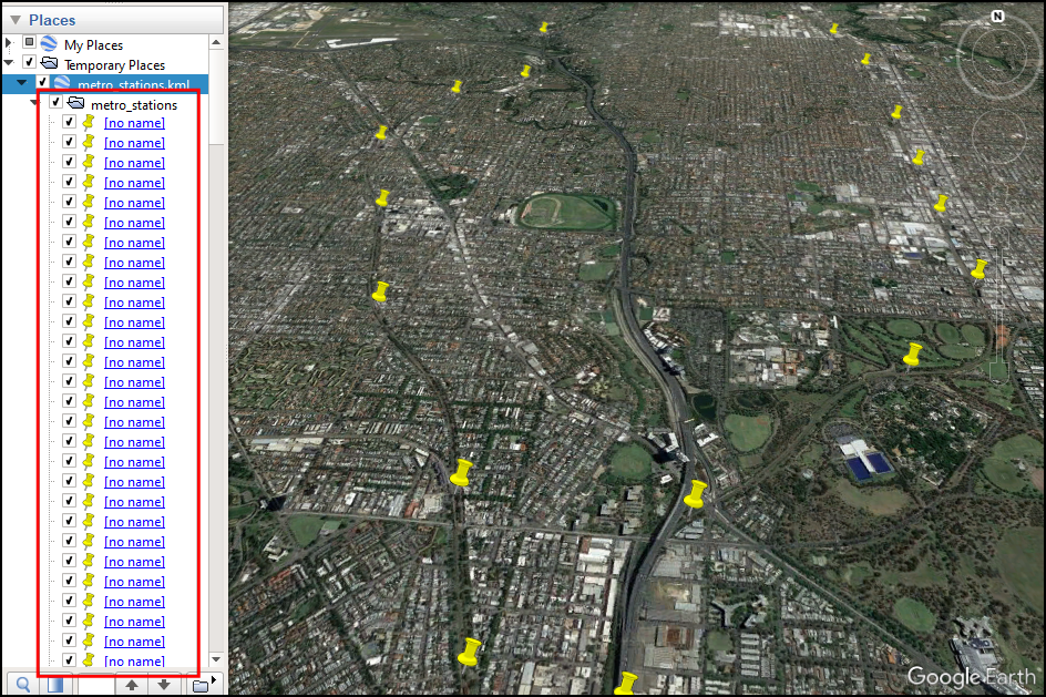
KML Export without NameField
While the above command works, you will detect that when you open up the resulting file in Google Earth, the placemarks for each feature doesn't have any labels. This is because the KML format expects a field called Name in the layer which is used as the label for each placemark. If your data layer does not have such a field, y'all tin can supply an alternate field proper noun that volition be used as labels using the -dsco pick. The metro_stations layer has a field named station which nosotros can use as the name field.
ogr2ogr -f KML metro_stations.kml spatial_query.gpkg metro_stations -dsco NameField=station 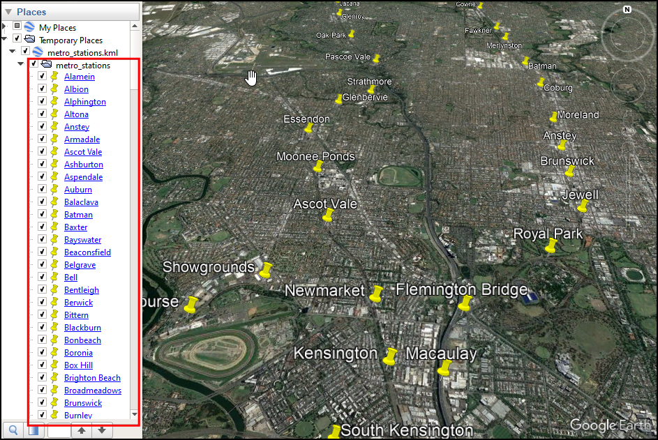
KML Export with NameField
Converting KML Files to Other Formats
The KML file format supports having multiple data layers within the same KML file. Nosotros will now learn how to extract a specific data layer and convert it to a shapefile. GDAL supports reading data from a URL using the Virtual File System. We tin can read a KML file from the internet using the vsicurl/ prefix.
ogrinfo /vsicurl/https://developers.google.com/kml/documentation/KML_Samples.kml 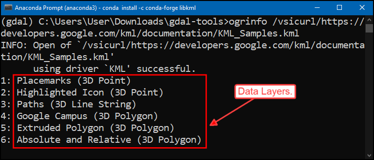
Permit's read the Paths layer
ogrinfo /vsicurl/https://developers.google.com/kml/documentation/KML_Samples.kml Paths 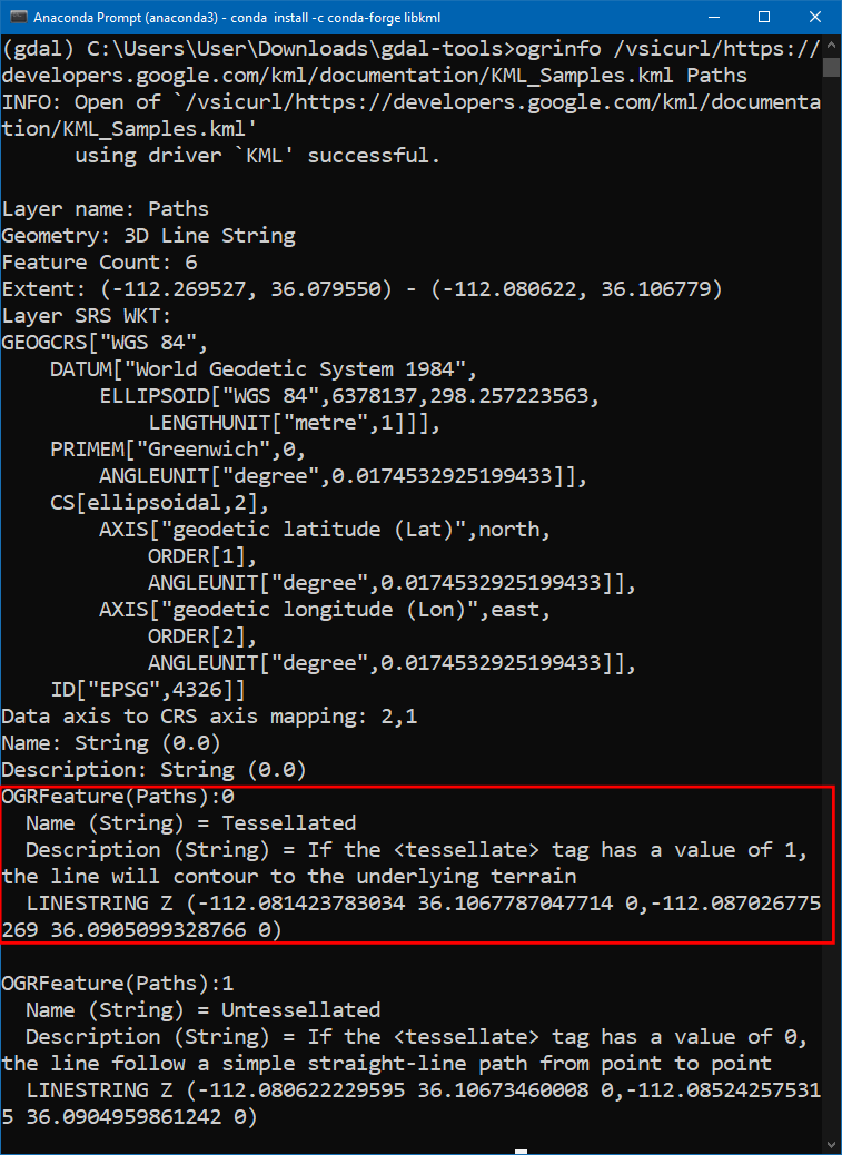
To extract the Paths layer from this KML file, we can use ogr2ogr command. The default options create many unwanted fields in the output. We can select a subset of the input fields using the -select choice.
ogr2ogr -f "ESRI Shapefile" paths.shp /vsicurl/https://developers.google.com/kml/documentation/KML_Samples.kml Paths -select "NAME,Clarification" 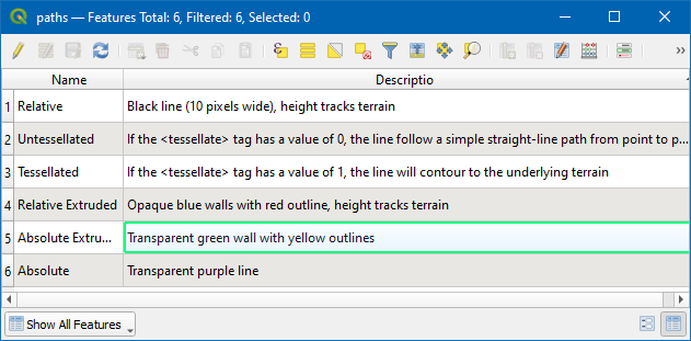
Y'all can also catechumen a KML layer to a CSV file. The GDAL CSV Driver is able to extract the geometry of features using the GEOMETRY layer cosmos choice. Let's convert the Placemark layer from the KML_Samples.kml to a CSV file with X, Y and Z columns extracted from the geometry.
ogr2ogr -f CSV points.csv /vsicurl/https://developers.google.com/kml/documentation/KML_Samples.kml Placemarks -lco GEOMETRY=AS_XYZ 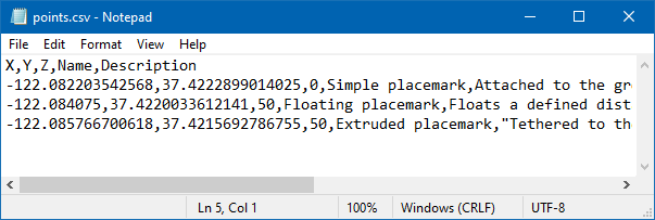
KML vs. LIBKML Drivers
If your GDAL binaries are compiled with support for the LIBKML Driver, information technology is preferable to use it over the KML driver. The LIBKML driver supports many more options and allows you to create fully featured KMLs.
Below is an example of information conversion using the LIBKML driver. To specify the name field, the LIBKML commuter uses an environment variable called LIBKML_NAME_FIELD that tin be specified with the --config selection
ogr2ogr -f LIBKML metro_stations.kml spatial_query.gpkg metro_stations --config LIBKML_NAME_FIELD station If your GDAL version has both KML and LIBKML drivers, OGR will prefer the LIBKML driver. To force OGR to use the KML driver for reading files, yous can add --config OGR_SKIP LIBKML to your command.
Using Virtual Layers
Like to GDAL, OGR besides supports Virtual File Format (VRT). Compared to the raster version, the OGR Virtual Driver is much more capable and can be used for on-the-fly information transformations. Multiple data layers can be combined into a single virtual layer using the XML-based .vrt format files. VRT files are besides used to configure reading tabular information into spatial data formats.
Read Geonames Files
Your information package contains 3 large text files from Geonames in the geonames folder. These are plain-text files in a Tab-Separated Values (TSV) format. Modify to the geonames directory.
cd geonames Let's try reading 1 of the files CA.txt - which has over 300K records of all placenames in Canada. To read this file, we demand to create a new file called CA.vrt with the following content. Relieve the file in the aforementioned geonames directory.
<OGRVRTDataSource> <OGRVRTLayer name="CA"> <SrcDataSource>CSV:CA.txt</SrcDataSource> <SrcLayer>CA</SrcLayer> </OGRVRTLayer> </OGRVRTDataSource> 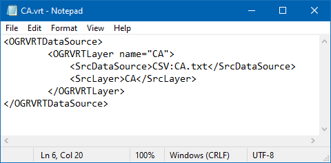
Let'south cheque if OGR can read the source text file via the newly created CA.vrt file.
ogrinfo -al -so CA.vrt 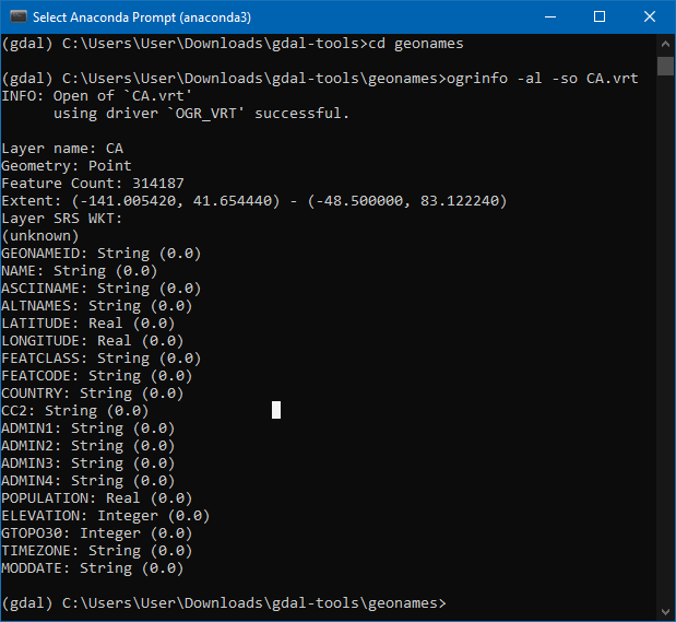
The ogrinfo command was able to successfully read the data and show usa the summary of the attributes as well as the total feature count. Note that OGR has congenital-in support for the geonames file format. So it was able to correctly detect the geometry columns without the states specifying information technology. For other datasets, you will take to specify the geometry columns explicitly via the <GeometryField> attribute in the VRT file.
Applying Filters
VRT format supports applying SQL queries on the source layer using the <SrcSQL> field. This allows us to create an on-the-fly filter that reads just a subset of the information. Update the CA.vrt with the following content.
<OGRVRTDataSource> <OGRVRTLayer name="CA"> <SrcDataSource>CSV:CA.txt</SrcDataSource> <SrcLayer>CA</SrcLayer> <SrcSQL>select * from CA where "FEATCLASS" = 'T'</SrcSQL> </OGRVRTLayer> </OGRVRTDataSource> 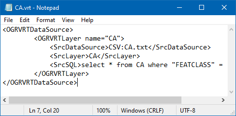
The VRT file now contains a SQL query to select merely the mountain features from the source file. Let's run ogrinfo over again and check the output.
ogrinfo -al -so CA.vrt 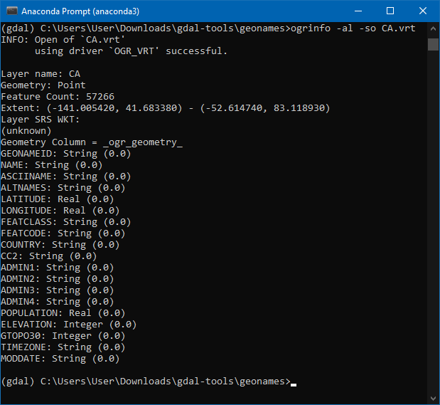
You will see that the output contains a subset of features, even though we never changed the source data.
Merging Files
The real ability of the VRT file format lies in its power to dynamically combine multiple data sources into a single data layer. We can adapt the previously created file and employ <OGRVRTUnionLayer> to create a single layer from the 3 carve up text files. Salvage the post-obit content into a new file named NA.vrt.
<OGRVRTDataSource> <OGRVRTUnionLayer name="NA"> <OGRVRTLayer name="CA"> <SrcDataSource>CSV:CA.txt</SrcDataSource> <SrcLayer>CA</SrcLayer> <SrcSQL>select * from CA where "FEATCLASS" = 'T'</SrcSQL> </OGRVRTLayer> <OGRVRTLayer name="MX"> <SrcDataSource>CSV:MX.txt</SrcDataSource> <SrcLayer>MX</SrcLayer> <SrcSQL>select * from MX where "FEATCLASS" = 'T'</SrcSQL> </OGRVRTLayer> <OGRVRTLayer proper noun="The states"> <SrcDataSource>CSV:US.txt</SrcDataSource> <SrcLayer>Us</SrcLayer> <SrcSQL>select * from Usa where "FEATCLASS" = 'T'</SrcSQL> </OGRVRTLayer> </OGRVRTUnionLayer> </OGRVRTDataSource> 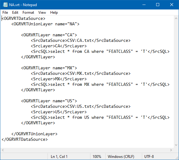
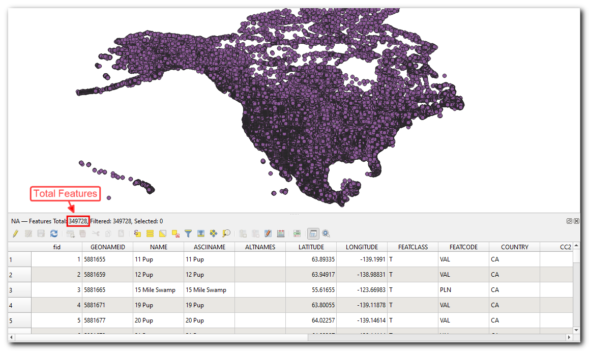
Let's now translate the NA.vrt to a GeoPackage using the ogr2ogr command.
ogr2ogr -f GPKG NA.gpkg NA.vrt -a_srs EPSG:4326 This operation requires a lot of processing and may have a few minutes. Y'all tin can add the
--config GDAL_CACHEMAX 512option to speed upward the process. Come across Tips for Improving Functioning department for more details.
This command reads all 3 text files, filters them for matching features, combines them and writes out a spatial layer containing all mountains in North America.
Information Credits
- Landsat: Landsat-8 paradigm courtesy of the U.S. Geological Survey. Paradigm downloaded from Google Deject Platform and pre-processed using Semi Automatic Classification Plugin from QGIS
- Globe at Night epitome: Credit: NASA World Observatory/NOAA NGDC. Earth at Night apartment hi-resolution map downloaded from NASA earth observatory
- William Mackenzie 1870 map of Southern India: out-of-copyright scanned map downloaded from Hipkiss's Scanned One-time Maps
- NAIP 2022 Aerial Imagery for California: The National Agriculture Imagery Program (NAIP). USDA-FSA-APFO Aerial Photography Field Office. Downloaded from NRCS
- London 1m DSM. Downloaded from Defra Data Services Platform. © Environment Agency copyright and/or database right 2022. All rights reserved.
- Melbourne Metro Stations: © 2022 The Urban center of Melbourne Open up Data Portal. Data provided by Metro Trains Melbourne
- Melbourne Confined and Pubs: © 2022 The Metropolis of Melbourne Open up Information Portal. Data provided by Census of State Apply and Employment (CLUE)

Source: https://courses.spatialthoughts.com/gdal-tools.html
Posted by: danieltrum1952.blogspot.com
0 Response to "How To Check If Gdal Is Installed"
Post a Comment